フーリエ級数と波動方程式

前回フーリエ変換による波動方程式の解を考えた。

今回はフーリエ級数を用いて波動方程式の初期値境界値条件を考える。

両端を固定した弦の動きを波動方程式で示すと、

$$
\frac{\partial^2 u}{\partial t^2} = c^2 \frac{\partial^2 u}{\partial x^2}
$$

ここで長さLの弦の両端が動かないとして、
$$
u(0, t) = u(L, t) = 0
$$

となる。この条件を境界条件という。

初期条件は

$$
u(x, 0) = f(x), \quad \frac{\partial u}{\partial t}(x, 0) = g(x)
$$

とする。いま、

$$ \sin\left(\frac{n \pi x}{L}\right) \cos\left(\frac{n \pi c t}{L}\right)$$

と

$$ \sin\left(\frac{n \pi x}{L}\right) \sin\left(\frac{n \pi c t}{L}\right)$$

は波動方程式の解であり、かつ初期条件と境界条件を満たす。

波動方程式の解の性質として、解の和は解であり、解のスカラー倍も解である。

よって一般解は

$$u(x, t) = \sum_{n=1}^\infty \left[ A_n \sin\left(\frac{n \pi x}{L}\right) \cos\left(\frac{n \pi c t}{L}\right) + B_n \sin\left(\frac{n \pi x}{L}\right) \sin\left(\frac{n \pi c t}{L}\right) \right]$$

と考えることができる。すなわち、

解のフーリエ級数展開
$$
u(x, t) = \sum_{n=1}^\infty \left[ A_n \cos\left(\frac{n \pi c t}{L}\right) + B_n \sin\left(\frac{n \pi c t}{L}\right) \right] \sin\left(\frac{n \pi x}{L}\right)
$$

である。ここでフーリエ係数A_nとB_nは初期条件と境界条件を考えて
$$
A_n = \frac{2}{L} \int_0^L f(x) \sin\left(\frac{n \pi x}{L}\right) dx, \quad
B_n = \frac{2}{n \pi c} \int_0^L g(x) \sin\left(\frac{n \pi x}{L}\right) dx
$$

である。

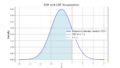
タイトル画像のコードです。(chatGPT産)

import numpy as np
import matplotlib.pyplot as plt
from matplotlib.animation import PillowWriter, FuncAnimation

# Constants
L = 1.0  # Length of the string
c = 1.0  # Wave speed
T = 2.0  # Duration for visualization
N = 5    # Number of Fourier modes

# Discretize space and time
x = np.linspace(0, L, 500)  # Space points
t = np.linspace(0, T, 200)  # Time points

# Initial displacement (f(x)) and velocity (g(x)) for the string
def f(x):
    return np.sin(np.pi * x)  # Initial displacement (single sine wave mode)

def g(x):
    return 0 * x  # Initial velocity (stationary string)

# Calculate Fourier coefficients
A_n = lambda n: 2 / L * np.trapz(f(x) * np.sin(n * np.pi * x / L), x)
B_n = lambda n: 2 / (n * np.pi * c) * np.trapz(g(x) * np.sin(n * np.pi * x / L), x)

# Compute string motion
u = np.zeros((len(t), len(x)))  # Initialize solution
for n in range(1, N + 1):
    A = A_n(n)
    B = B_n(n)
    u += (A * np.cos(n * np.pi * c * t[:, None] / L) +
          B * np.sin(n * np.pi * c * t[:, None] / L)) * np.sin(n * np.pi * x[None, :] / L)

# Create the animation
fig, ax = plt.subplots(figsize=(10, 6))
line, = ax.plot([], [], label="String Motion")
ax.set_xlim(0, L)
ax.set_ylim(-1.2, 1.2)
ax.set_xlabel("Position (x)")
ax.set_ylabel("Displacement (u)")
ax.set_title("String Motion Over Time")
ax.legend()
ax.grid()

# Update function for the animation
def update(frame):
    line.set_data(x, u[frame, :])
    ax.set_title(f"String Motion at t = {t[frame]:.2f}s")
    return line,

# Create animation
ani = FuncAnimation(fig, update, frames=len(t), interval=50, blit=True)

# Save as GIF
output_path = "string_motion.gif"
ani.save(output_path, writer=PillowWriter(fps=20))
plt.close()
print(f"GIF saved to {output_path}")